What Are Often Used on Graphs to Show Statistical Comparisons?
 Researchers rely heavily on sampling.
It's rarely possible, or even makes sense, to measure out every single person of a population (all customers, all prospects, all homeowners, etc.).
But when you use a sample, the boilerplate value yous observe (e.g. a completion charge per unit, boilerplate satisfaction) differs from the actual population boilerplate.
Consequently, the differences between designs or attitudes measured in a questionnaire may be the result of random noise rather than an actual departure—what's referred to as sampling error.
Understanding and appreciating the consequences of sampling error and statistical significance is one thing. Conveying this concept to a reader is another challenge—especially if a reader is less quantitatively inclined.
Picking the "correct" visualization is a balance between knowing your audience, working with conventions in your field, and not overwhelming your reader. Hither are half-dozen ways to indicate sampling error and statistical significance to the consumers of your enquiry.
1. Confidence Interval Mistake Confined
Confidence intervals are one type of error bar that tin can be placed on graphs to show sampling fault. Confidence intervals visually testify the reader the near plausible range of the unknown population average. They are usually xc% or 95% by convention. What's squeamish about conviction intervals is that they act as a shorthand statistical test, fifty-fifty for people who don't understand p-values. They tell yous if two values are statistically dissimilar along with the upper and lower bounds of a value.
That is, if there's no overlap in confidence intervals, the differences are statistically pregnant at the level of confidence (in most cases). For example, Figure i shows the findability rates on two websites for different products along with 90% conviction intervals depicted equally the black "whisker" error bars.

Effigy ane: Findability rates for two websites. Black fault bars are xc% confidence intervals.
Almost 60% of 75 participants found the sewing machine on website B compared to only four% of a different group of 75 participants on website A. The lower purlieus of website B'due south findability rate (49%) is well to a higher place the upper boundary of website A'south findability rate (12%). This difference is statistically meaning at p < .10.
Yous tin likewise meet that the findability rate for website A is unlikely to always exceed 15% (the upper boundary is at 12%). This visually tells you lot that with a sample size of 75, it's highly unlikely (less than a v% risk) that the findability rate would ever exceed xv%. Of course, a 15% findability charge per unit is abysmally depression (significant roughly simply i in seven people will ever find the sewing machine).
This is my preferred method for displaying statistical significance, but fifty-fifty experienced researchers with strong statistics backgrounds accept trouble interpreting conviction intervals and they aren't always the all-time option, equally we run into below.
2. Standard Error Fault Confined
Another blazon of error bar uses the standard error. These standard mistake error bars tend to be the default visualization for academia. Don't be confused past the proper noun—standard mistake fault bars aren't necessarily the "standard." The name is due to the fact that they display the standard error (which is an approximate of the standard divergence of the population mean). For example, Figure two shows the perceived ease for a task on four retail websites using the Single Ease Question (SEQ) and the standard error for each.

Figure 2: Perceived ease (using the SEQ) with standard error error bars for iv retail websites.
The standard error is often used in multiple statistical calculations (eastward.g. for calculating confidence intervals and statistical significance) so an advantage of showing merely the standard error is that other researchers can more than hands create derived computations.
The main disadvantage I see is that people still interpret it as a confidence interval, merely the not-overlap no longer corresponds to the typical thresholds of statistical significance. Showing one standard error is actually equivalent to showing a 68% conviction interval. The 90% confidence intervals for the aforementioned data are shown in Effigy 3. You tin can meet the overlap in R1 and R2 (significant they are NOT statistically different); whereas the non-statistical difference is less easy to spot with standard error error bars (Figure 2).
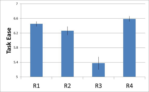
Effigy iii: Perceived ease and 90% conviction intervals for four retail websites.
3. Shaded Graphs
Error bars of any kinds tin add a lot of "ink" to a graph, which can freak out some readers. A visualization that avoids error confined is to differ the shading on the bars of a graph that are statistically significant. The dark red bars in Effigy iv show which comparisons are statistically significant. This shading can be done in colour or in black-and-white to be printer friendly.
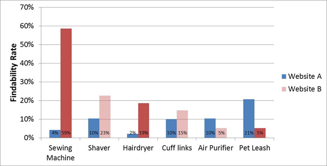
Figure 4: Findability rates for two websites; the dark ruby-red bars betoken differences that are statistically pregnant.
iv. Asterisks
An asterisk (*) or other symbol can indicate statistical significance for a small number of comparisons (shown in Figure five). We've as well seen (and occasionally use) multiple symbols to indicate statistical significance at ii thresholds (oft p
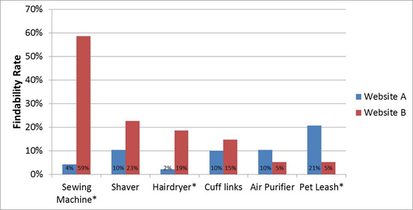
Figure 5: Findability rates for ii websites; asterisks indicate statistically meaning differences.
5. Notes
It'southward often the example that then many comparisons are statistically meaning that any visual indication would exist overwhelming (or undesired). In those cases, a note depicting significance is ideal. These notes tin be in the footer of a table, the caption of an image (equally shown in Effigy 6), or in the notes department of slides.

Figure 6: Findability rates for two websites. Sewing Auto, Hairdryer, and Pet Leash findability rates are statistically dissimilar.
six. Connecting Lines and Hybrids
When differences aren't contiguous an alternative approach is to include connecting lines as shown in Figure 7 below. It shows 8 weather in a UX research study using three measures (satisfaction, confidence, likelihood to purchase). Iii differences were statistically unlike as indicated by the connecting lines. The graph also includes 95% confidence intervals and notes in the caption.
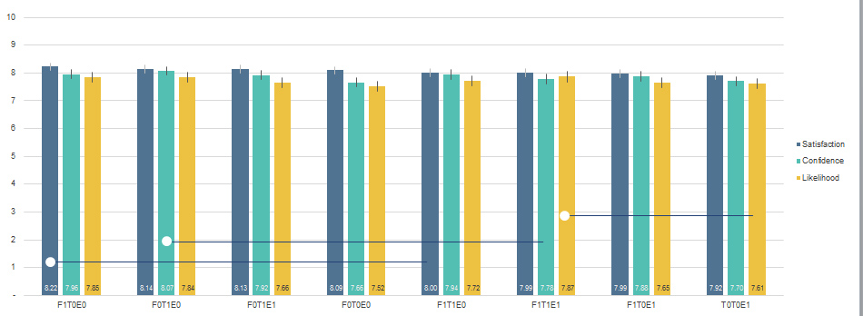
Figure 7: Mean satisfaction, confidence and likelihood to purchase across viii conditions. Error bars are 95% confidence intervals. Connecting lines show statistical differences for conditions: satisfaction F1T0E0 vs. F1T1E0; confidence F0T1E0 vs F1T1E1; and likelihood to purchase F1T1E1 vs. T0T0E1.
Source: https://measuringu.com/visualize-significance/
0 Response to "What Are Often Used on Graphs to Show Statistical Comparisons?"
Post a Comment